Introduction to matching¶

Build the graph¶

First, let’s build a GraphInterface object

model = g007();
    initialGraph = GraphInterface();
    initialGraph.readModel(model);
    initialGraph.createAdjacency();

A plot of the original graph can be seen in Basic functionality.

Match with Weighted Elimination¶

Let’s perform a matching using the Weighted Elimination algorithm. It maintains the set of equations which have only one unknown, unmatched veriable and in each step it adds to the matching the cheapest calculation, until the set is depleted

First, create a copy of the initial graph

graphWE = copy(initialGraph);

Then ,create a matcher object

matcher = Matcher(graphWE);

Perform the matching

matching = matcher.match('WeightedElimination');

Plot the result.

plotter = Plotter(graphWE);
plotter.plotDot('matchedWE');

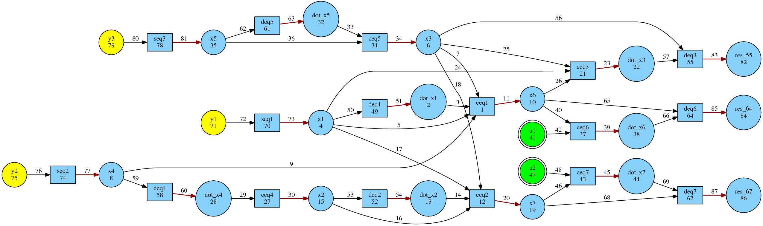
Notice how the known variables are now shown in blue. Also the matching procedure has specified a direction for the graph edges. The graph is now fully directed. Residual variables have been added onto the redundant constraints.

Display the edges of the matching set and compare with plot

disp(matching);

73    77    81    51    60    30    63    34    11    23    39    54    20    45

Match with BBILP¶

Now let’s use the BBILP algorithm to generate matching sets. In order to have fault isolation capabilities, it is beneficial to create as many matching sets, each providing a different fault signature. To that goal, we will generate as many PSO sets as possible and match them using BBILP. BBILP generates the cheapest valid matching for the given PSO.

Once again, copy the original graph

graphBBILP = copy(initialGraph);

Now, create a SubgraphGenerator object, which has the funcitonality to create the multiple PSOs.

SG = SubgraphGenerator(graphBBILP);

It uses the Fault Diagnosis Toolbox to generate the PSO set: namely the set of MTESs. For this example, there are 10 MTESs.

SG.buildLiUSM();
SG.buildMTESs();
PSOSet = SG.getMTESs();

The SubgraphGenerator will read each MTES and create a subgraph with only those equations, pruning any known variables.

PSOSubgraphs = GraphInterface.empty;
h = waitbar(0,'Building MTES Subgraphs');
for i=1:length(PSOSet)
    waitbar(i/length(PSOSet),h);
    PSOSubgraphs(i) = SG.buildSubgraph(PSOSet{i},'pruneKnown',true,'postfix','_MTES');
    PSOSubgraphs(i).createAdjacency();
end
close(h)

A Matcher object for each subgraph is created to handle the matching procedure.

matchers = Matcher.empty;
h = waitbar(0,'Examining PSOs');
for i=1:length(PSOSubgraphs)
    fprintf('\n');
    disp('Examining another PSOs')
    tempGI = PSOSubgraphs(i);
    matchers(i) = Matcher(tempGI);
    matching = matchers(i).match('BBILP','branchMethod','cheap');
    waitbar(i/length(PSOSubgraphs),h);
end
close(h)

The resulting matchings sets can be printed with the following commands.

fprintf('\nResulting valid matchings:\n');
for i=1:length(matchers)
    disp(matchers(i).matchingSet);
end

Let us examine two specific matchings. First the edge set

3    26    34    57    63    73    77    81

Giving the directed subgraph

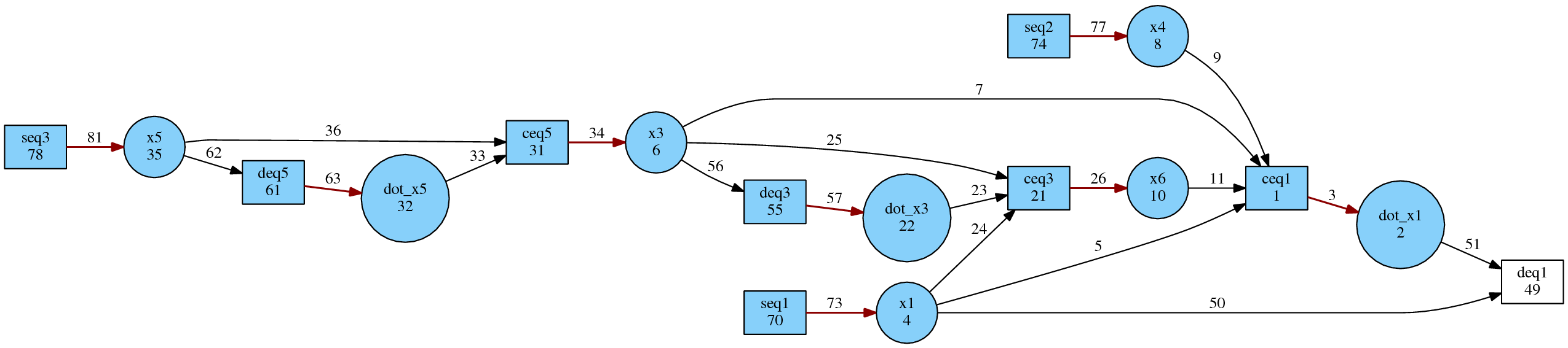
The corresponding order of evaluations is, in pairs of equation/variable:

1. seq1 -> x1
2. seq2 -> x4
3. seq3 -> x5
4. deq5 -> dot_x5
5. ceq5 -> x3
6. deq3 -> dot_x3
7. ceq1 -> x6
8. ceq1 -> dot_x1

Forming a residual with equation deq1. Direct, single-equation evaluations were required for the generaiton of this residual.

Another matching set is

3    23    39    56    65    73    77

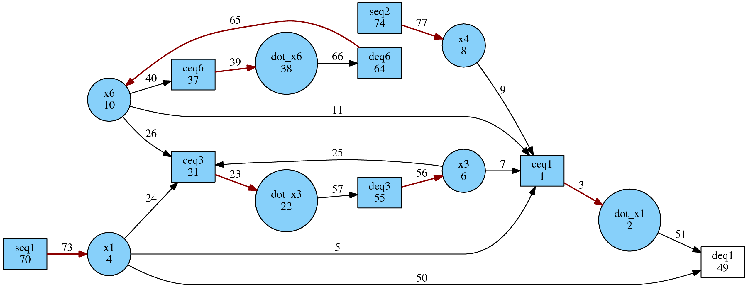
The corresponding order of evaluations is:

1. seq1 -> x1
2. seq2 -> x2
3. ceq6 -> dot_x6, deq6 -> x6
4. ceq3 -> dot_x3, deq3 -> x3
5. ceq1 -> dot_x1

Again, forming a residual generator at deq1. However, this time there exist Strongly Connected Components in the resulting directed graph. Namely, the evaluations 3 and 4 require an ODE solver to obtain the values of x6 and x3.

Whether such a residual generator can be implemented in a diagnostic system is the decision of the designer.